Create a sphere, specify the physical conditions for your simulation, view the pressure coefficient contours on the sphere, and generate an XY plot.

Goals

In this tutorial, you will learn how to:

• Create a quadrant of a sphere and use symmetry planes to generate results for a full sphere
• Rotate geometry around an axis
• Specify physical conditions for a simulation, including the velocity of air flowing around the sphere and the properties of the outer surface of the sphere
• Specify meshing parameters
• Generate a color map (contours)
• Create an XY plot
• Save your simulation to a file

Assumptions

1. You have activated the Caedium Builder and Caedium Panel Flow add-ons, or Caedium Professional.
2. You are familiar with Caedium essentials.

Create a Sphere Quadrant

Select the Geometry Tool Palette. Select the Volumes->Sphere tool. Turn off the Decompose property in the Properties Panel, enter a Radius of 5, and enter a Sector of 90. Press Enter on the keyboard to apply the changes to the Properties Panel.

The Decompose option instructs Caedium to split the sphere into six four-edged faces. This option is useful in simplifying the meshing process.

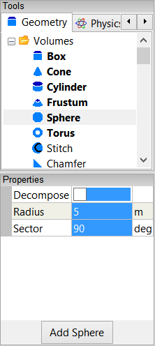
Click Add Sphere and select Done to create a sphere quadrant in the View Window.

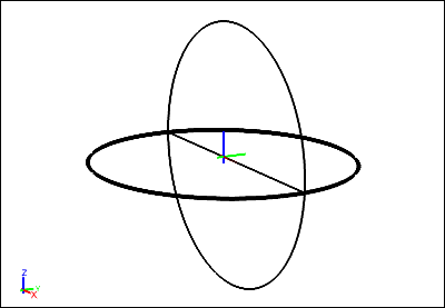
Rotate the Quadrant Around the Y-Axis

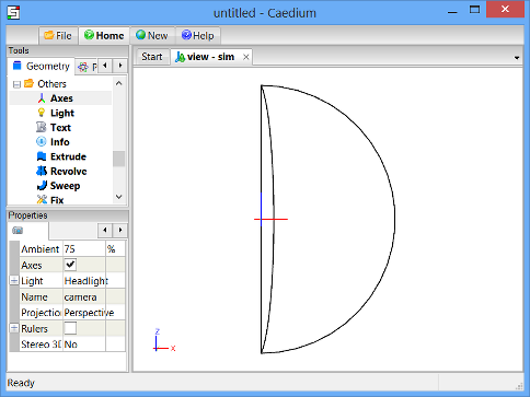
It is customary to specify the flow direction in the X-direction. In this step you will rotate the sphere quadrant so that its straight edge is aligned parallel to the X-axis. To do this, you need to rotate the sphere quadrant about the center of its straight edge. This requires that you create axes at the center of that edge, which also coincides with the origin in this case.

Drag and drop the Others->Axes tool onto the background of the View Window. Double-click sim in the Select dialog and select Done to create axes (axes).

Axes are created at the origin by default. In this case, the origin is at the center of the straight edge of the sphere quadrant.

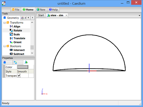
To rotate the sphere quadrant around the Y-axis, select the Transforms->Rotate tool. In the Properties Panel set Y to -90 and press Enter on the keyboard to apply the changes.

A positive rotation indicates a clockwise rotation around a positive coordinate direction. Conversely, a negative rotation indicates a counterclockwise rotation around a positive coordinate direction. This convention is commonly referred to as the right-hand rule.

Drag the Transforms->Rotate tool and drop it directly onto the axes you created in the View Window. Select Set Axes to rotate the sphere quadrant around those axes. Right-click on an edge of the sphere quadrant (which in this case will select the quadrant volume) and select Done to rotate the quadrant around the Y-axis.

Specify the Fluid Conditions

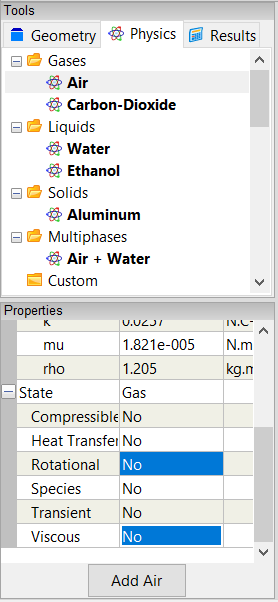
Select the Physics Tool Palette. Select Substances->Air. The Properties Panel will show the default properties for air. To enable incompressible, irrotational, inviscid flow, set the 5 properties under State (Compressible, Heat Transfer, Rotational, Transient, and Viscous) to No (if they are not set to No already).

Drag and drop the Substances->Air tool onto the background of the View Window, which represents the simulation (sim). Double-click sim in the Select dialog and select Done to set air as the fluid surrounding the sphere.

Select the Conditions->Linear Velocity tool. In the Properties Panel set the Velocity to [1 0 0].

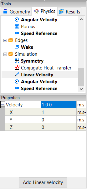
Drag and drop Conditions->Linear Velocity onto the background of the View Window. Double-click sim in the Select dialog and select Done to set the velocity of the air at 1 m/s in the X-direction.

Define the Symmetry Planes for the Sphere

Caedium will calculate results on the sphere quadrant. However, since a sphere is a symmetrical shape, you can use the symmetry planes tool to see results for a whole sphere. Using symmetry allows you to get results faster and using less computing resources.

Select the Conditions->Symmetry tool. Select Y+Z next to Planes in the Properties Panel.

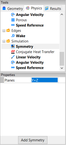
Drag and drop the Conditions->Symmetry tool onto the background of the View Window and select Done to set Y and Z as the symmetry planes.

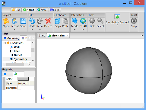
To see the full sphere, select the View tab in the Properties Panel and turn on the Symmetry property. Click on the Fit All icon in the Toolbar so that you can see the whole sphere in the View Window.

To shade the sphere, right-click on one of its edges, select the outer face of the sphere in the Select dialog (both of the sphere's edges you see in the View Window will be highlighted), click OK, and select Properties. Turn off the Transparent property in the Properties Panel to shade the sphere.

Set the Properties of the Outer Surface of the Sphere

Drag and drop the Conditions->Wall tool onto the outer face of the sphere. Select the outer face of the sphere in the Select dialog, click OK, and select Done to create a wall on the outer surface of the sphere.

A wall is a solid surface through which fluid cannot flow.

Specify Meshing Parameters

Select the Conditions->Accuracy tool. Select High for the Accuracy in the Properties Panel.

Drag and drop the Conditions->Accuracy tool onto the outer face of the sphere. Select the outer face of the sphere in the Select dialog, click OK, and select Done to set the accuracy of the calculation you want on the sphere.

You can experiment with selecting the Low and Medium accuracies at the end of this tutorial to see the effect that these settings have on your results. To do this, right-click on the outer face of the sphere, select the outer face in the Select dialog, click OK and select Properties. Select the Face tab in the Properties Panel and select a different Accuracy from the pulldown menu.

Calculate the Pressure Coefficient on the Sphere

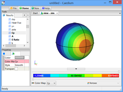
Select the Results Tool Palette. Drag and drop the Scalar Fields->Cp tool onto the outer face of the sphere in the View Window. Select the outer face in the Select dialog, click OK, and select Color Map to create contours of pressure coefficient on the sphere.

The pressure coefficient is a dimensionless number that relates pressure changes to the surrounding field pressure.

To rotate the view, left-click-and-drag the mouse in the View Window.

Create an XY Plot of the Pressure Coefficient on the Sphere

Drag and drop the Scalar Fields->Cp (pressure coefficient) tool onto the edge of the sphere highlighted in the diagram below.

Double-click the edge in the Select dialog and select XY Plot.

Note that the edges may have different names in your example, so use the diagram above as a guide for the edge to be selected.

Save the Simulation

In the Toolbar click the Save icon . Select the location to save your simulation, specify a File name (e.g., flow-over-sphere) and select Caedium (*.sym) as the file type (if it is not already selected). Click Save to save the sym file.

Compare your Results with Theory

You can compare the results of your simulation with theoretical calculations of pressure coefficient on a sphere. See the Fluid Flow Around a Sphere: Theory Comparison tutorial for detailed instructions.